
Goal of this Article
With this article, we hope to detail our process as members of Bruin Sports Analytics to work towards getting a well-done research paper completed, with guidance given by our club advisor, Professor Almohalwas of the UCLA Statistics department. We wish to detail our journey, and all the lessons we have taken from each one to move us closer to completing our desired task. In hopes of creating a paper worthy of being published in an official sports analytics journal, we have decided to take more time in working towards our final result. However, we have decided to write this extended article to provide a checkpoint of where currently stand in hopes for others to get inspired to do research as an undergrad, and learn more about the interesting attempts we have tried to solve our problem.
Predicting NBA Free Agent Salaries
Introduction Relevance
Front ofSces and player agents alike would beneSt from a model that can assess a free agent’s true value given the player’s performance in an array of statistical categories. In 2016, teams were clearly unsure how much free agents were actually worth due to the increased salary cap (it increased by over $24 million). As the salary cap continues to increase with the in]ux of more league revenue from television contracts, this problem will continue. Our research attempts to lay the groundwork for a tool to accurately gauge the true worth of a player’s on-court contributions in relation to the salary cap.
Background

More so than any of the other big four American sports, the NBA is a superstar-driven league. Every championship team this millennium aside from the 2004 Detroit Pistons and the 2011 Dallas Mavericks have featured at least two bona-Sde superstars. This trend has been accentuated by the 2010-2014 Miami Heat featuring three superstars and the current Golden State Warriors featuring four.
By far the easiest way to acquire superstars is through signing a superstar through free agency, which requires no sacriSce of time or assets except money of course. The player and his new team need only agree to a maximum contract, without the team compensating his previous team. Thus, signing free agent superstars is, on paper, the easiest way to get a superstar.
The NBA CBA designates a salary cap and a maximum contract, which complicate the signing of multiple high-salary superstars while keeping a strong roster of complementary players. This leaves little to no room for overpaying players - every dollar counts. Thus, there is a need for a model that can analyze statistics to accurately predict any player’s appropriate salary for the next season, a tool which can help teams avoid overspending and help free agents know their clients’ worth.
Understanding Contracts and Free Agency
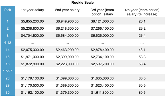
First round draft picks enter the league on two-year guaranteed contracts dictated by the CBA and its “rookie scale”. The rookie scale outlines how first rounders’ pay is based on a range tied to the salary cap in their draft year. This means players on rookie contracts are paid based on draft position, NOT on-court performance.
This rookie scale makes players on rookie contracts irrelevant to our research, and thus we removed these players from our data. Players like Donovan Mitchell (13th pick) and Kyle Kuzma (27th pick) have greatly outperformed their draft positions’ salaries while other players (busts) would underperform. Either way, both types of players would damage our model.
Methodology Organizing the Data
We obtained player metrics (both basic box-score and advanced numbers) from basketball- reference.com for players from the 2013-2014 through 2016-17 season. These metrics included the player’s Per Game and Advanced statistics, as these statistics do an adequate job of detailing the skill of a particular player. Each player was matched with average salary data for the corresponding player for the next season via spotrac.com. Our reason for using the next season’s salary was so that the model would be trained to predict player salary in the following season based on their performance in the previous season.
Once we had a dataframe of four seasons, we decided to optimize our data to focus our attention on players who were relevant over the course of an NBA season. Thus, we cleaned the data by removing duplicates and players who played less than 25 games in a season. These are generally players who are either injured or do not have much impact in games. In the case that a player was injured during the season, it would not make sense to predict their salary based on the performance from a season in which they were injured. Also, players that are generally unproductive when they are on the ]oor often bounce around teams on shorter contracts and thus have a greater variability in salaries over seasons. Cases like these could affect the model unfavorably.
Another step taken to clean the data for the model was to take out players on rookie contracts. As stated earlier, when a player is on a rookie contract, their salaries are set in stone for a certain amount of years. This means that predicting a player’s salary while on a rookie contract would be futile, since their salaries are set in stone for a Sxed amount of years after they are drafted, and are not based on performance.
Finally, we had to re-examine the goal of this project, which was to create a statistically valid model that could predict NBA player salaries for next season, the 2018-19 season. To do this, we decided to train the model on predicting player salaries for the 2017-18 season based on player performance in the 2016-17 season. We found that using the larger dataset of data from the previous seasons (2013-16) posed some issues in our methodology, namely in that the “local model” with just one season’s worth of data was more accurate.
Interesting Notes
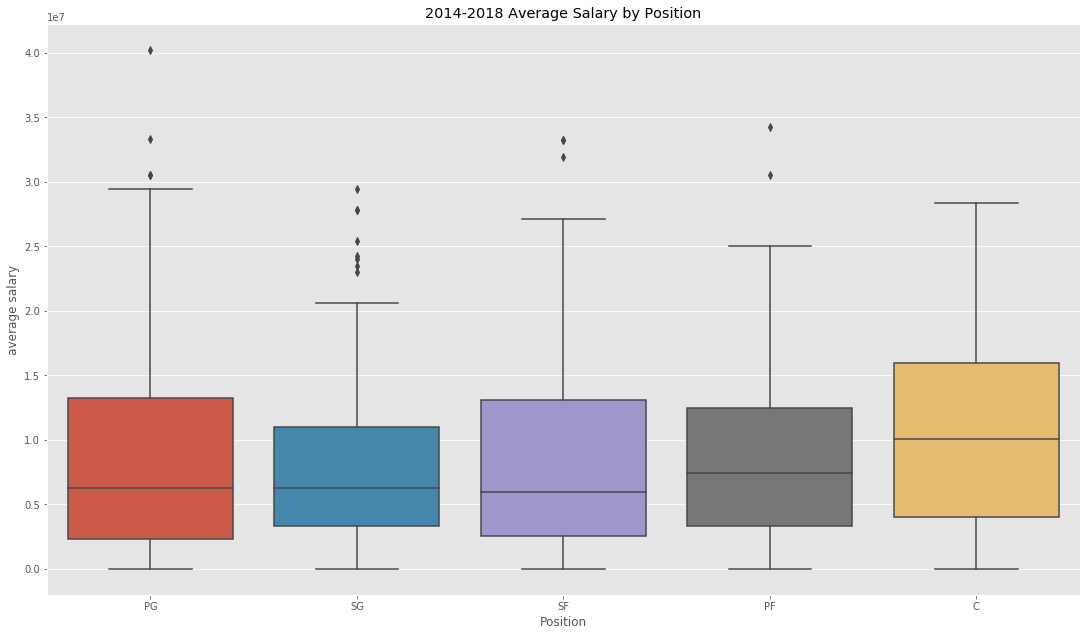
Once the data had been prepared, one of the first statistics we looked at was whether there was a signiScant difference in terms of average salary by player position.
To our surprise, after running a One-way ANOVA test comparing whether the average salary between groups was different, we concluded no signiScant difference between position thus did not add this factor into our multiple linear regression model.
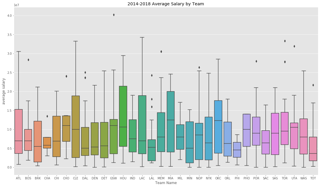
Another factor we explored was if playing for a speciSc team impacted the type of salary a player is expected to get.
After performing another another ANOVA test, there was a signiScant difference in terms of average salary by Team. However, after performing Post-hoc Tukey’s test to discover which pair was signiScant and adding that to our model, it also proved insigniScant compared to our other variables.

An Attempt to Create our Own Statistic
One of the other aspects that we worked on was creating a new statistic that we could eventually use in our regression model. The goal was to create a metric that would quantify how much a player was overachieving or underachieving with respect to their contract. Our belief was that a player who was underpaid would eventually see a pay raise in their next contract and a player that was underperforming would more than likely have to take a pay cut.
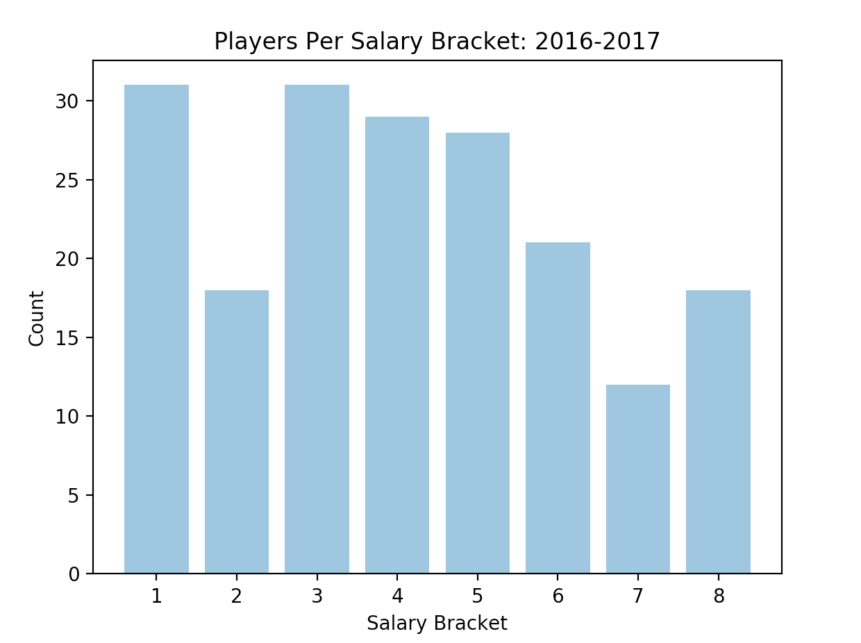
The first step in creating this new metric was to place the players into salary brackets according to how much they were being paid. We worked with the 2016-2017 player data and used their next year’s salary (2017-2018 season) to place them into salary brackets. We chose to have eight different salary brackets, where bracket eight represented players who received a max level contract, which was over 21% of the salary cap. The lowest bracket belonged to players on a minimum contract and from there the brackets went up in increments of roughly 3-4% of the overall cap. The following chart displays the distribution of players in each of the eight salary brackets.
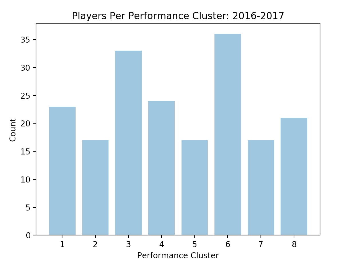
After assigning each of the players in the 2016-2017 season into a salary bracket, the next step was to group the players into clusters based on their performance. We used the K-Means clustering algorithm to create the groups. We chose to use a k-value of 8, because we wanted to be consistent with the number of salary brackets that we had previously created. After running the K- Means algorithm, each player was assigned into a performance cluster from one to eight. The eighth performance cluster represented the top performing players in the league and not surprisingly contained players like Lebron James, Stephen Curry, and Russell Westbrook. The chart below highlights the number of players in each of the respective performance clusters based on the 2016-2017 player data.
After assigning each player a performance cluster and a salary bracket, we had the information needed in order to create our new metric, which we called over/under. The formula for over/under was the following:
over/under = performance cluster - salary bracket
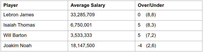
A positive over/under score meant that the player was outperforming their contract and was in line for a pay raise. Conversely, a negative over/under score represented a player that was underachieving and was most likely due for a decrease in pay in their next contract. The chart below shows a few players from our 2016-2017 dataset and their over/under score.
As shown, Lebron James, who belongs to both the highest performance cluster and highest salary bracket, has an over/under score of 0 which means that he should see similar pay in his future contract. In the cases of the Isaiah Thomas, who was an MVP candidate, and Will Barton, a sixth man of the year candidate, both had some of the highest over/under scores, which makes sense because they both signiScantly outperformed with respect to their contract. Joakim Noah achieved a negative score because of his limited production even though he belonged to such a high salary bracket.
Overall, after adding the over/under statistic into our regression model, we received an R^2 value of 82%, which was one of the best models that we had produced. However, the issue was that the over/under statistic relied on know the next year’s player salary, which was not possible if you were working with the most current NBA season. One way that we will use to solve this issue is by scaling the years back when calculating a player’s salary bracket. This would mean that for example with the 2016-2017 player data we would use the 2016-2017 player salary and not the 2017-2018 player salary. We also tried to use just the performance cluster metric for each player in a model and see if that had any statistical signiScance, but unfortunately it did not. Going forward there are numerous aspects that we can tune such as changing the number of performance clusters/salary brackets and scaling the salary years back in order to create a new metric that may improve our eventual regression model.
Final Variable Selection & Model Creation
Since we decided a multiple linear regression model would do the job in predicting average salary given a combination of various statistics, we had to require our model follow a large number of assumptions in order draw adequate conclusions. To begin with, we had to ensure that the player salaries were as close to normally distributed as possible. Average salary’s Gaussian Kernel Density estimation shape was greatly skewed but after applying the square root transformation, the assumption of normality was satisfied. Had this transformation not been applied, the standard errors would have been biased leading to faulty conclusions.
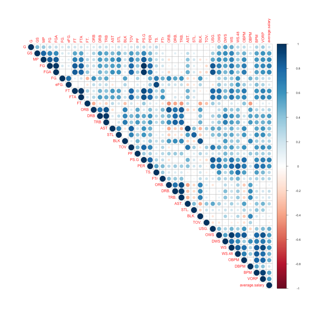
Next, we took a look at how the variables correlated with each other to better understand relationships.
When analyzing data as large as this, it is vital to view how the other statistics interact with average salary (the far right column). Next, for the variables which correlate greatly, you need to check how they correlate with each other. By checking for possible multicollinearity, we can avoid adding variables into our model which give the same information and just choose the one who provides us with the most information. For instance, the number of free throws made per game and free throw percentage tell nearly the same story in how a player performs at the line.
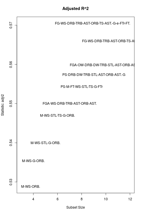
Next, we decided to use a powerful function within R, regsubsets, for regression subset selection which basically Snds the best combination of variables at various subset sizes in terms of a given criterion. We decided Adjusted R^2 was an adequate criteria to base our ability to explain average salary.
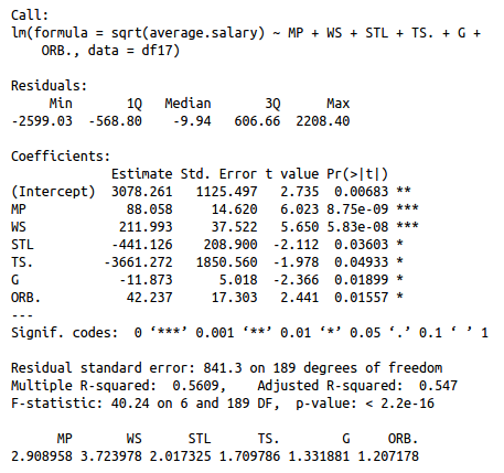
Our task then became selecting the subset which provides the highest adjust R^2 and cutting the model down while taking VIF into account. The variance in]ation factor of a variable gives us a sign of multicollinearity which we obviously want to avoid from our model. Finally, we worked our model down while keeping VIF of each variable under 5 to obtain:
We noticed that Minutes played per game, Win Shares, Steals per game, True Shooting %, Games played in the season, and offensive rebound % proved the most signiScant variables in predicting average salary according to this model. When checking for validity of a model, diagnostics must be examined.
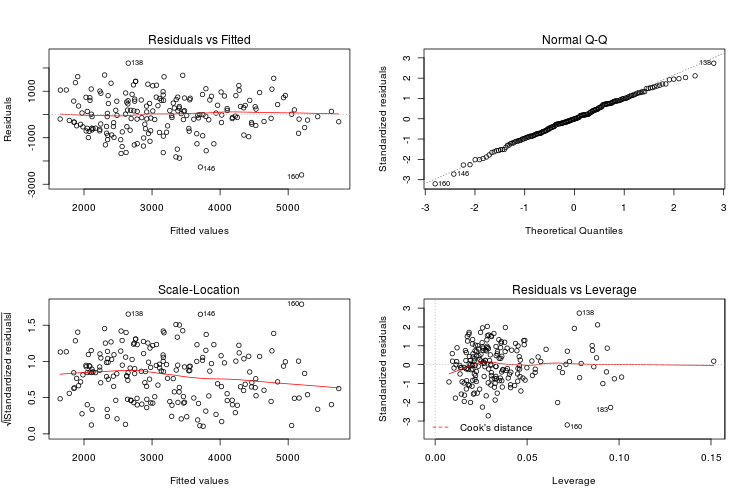
These four plots prove to us that our assumptions of normality and constant variance are all satisfied meaning that the conclusions we draw from the model can be taken seriously.
The model is nowhere near perfect yet, it has a low adjusted R^2, and some of the coefScients are negative when intuitively should be positive. We are still in progress to rework the regression model to raise our adjusted R^2 and explore different interactions between variables. However, we were able to satisfy all model assumption which at least gives a checkpoint to build off of as we begin to tune or rework this project.
Results
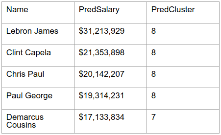
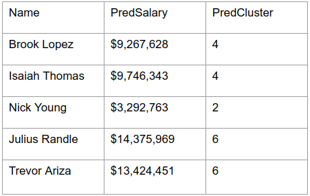
Based off this model for predicting 17-18 salaries, we decided to approximate what free agents for the 18-19 season should earn. Since the salary cap for the 18-19 season is so close to the 17-18 season, we decided to reuse this model to create approximate predictions.
Some top performers:
Editor's Picks
Not too shabby, but there’s so much more to go with the project if we want to improve our accuracy.
Next Steps
We are currently working with the professor on obtaining a model using Principal Component Analysis, and also exploring unsupervised methods to help create predictions on data with no attached labels. We also will try to incorporate more statistics such as offensive and defensive rating to hopefully give us more insight into detailing what a player is worth. Additionally, we will working to create extra statistics, such as our performance cluster and another which takes into account previous years.
We hope to one day predict full contracts with contract length attached, and possibly a web application for people to easily check a player’s worth in terms of what they deserve in salary against what they are currently earning.
Conclusion
This piece was just an update of where we are at so far, and to hopefully lay out a foundation on which we or others can build upon. All of our data from 2011-2017 of player’s perGame, advStats, salaries, free agent lists, etc is all our our github for you to use. Working towards getting this project completed has been an extremely rewarding experience, allowing us to get closer with our club members and working with our club advisory. It is highly recommended if you ever want to work towards solving a difficult problem and doing something you’re passionate about.